

K-means clustering is an unsupervised algorithm that is used in customer segmentation applications. In this algorithm, we try to form clusters within our datasets that are closely related to each other in a high-dimensional space.
Load the Datasets
from sklearn.datasets import load_digits

digits_data = load_digits().data
Output:
array([[ 0., 0., 5., ..., 0., 0., 0.], [ 0., 0., 0., ..., 10., 0., 0.], [ 0., 0., 0., ..., 16., 9., 0.], ..., [ 0., 0., 1., ..., 6., 0., 0.], [ 0., 0., 2., ..., 12., 0., 0.], [ 0., 0., 10., ..., 12., 1., 0.]])
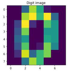
Each handwritten digit in the data is an array of color values of pixels of its image. For better understanding, let's print how the data of the first digit looks like and then display its's respective image
import matplotlib.pyplot as plt

print("First handwritten digit data: ", digits_data[0])
sample_digit = digits_data[0].reshape(8, 8)
plt.imshow(sample_digit)
plt.title("Digit image")
plt.show()
Output:
First handwritten digit data: [ 0. 0. 5. 13. 9. 1. 0. 0. 0. 0. 13. 15. 10. 15. 5. 0. 0. 3.
15. 2. 0. 11. 8. 0. 0. 4. 12. 0. 0. 8. 8. 0. 0. 5. 8. 0.
0. 9. 8. 0. 0. 4. 11. 0. 1. 12. 7. 0. 0. 2. 14. 5. 10. 12.
0. 0. 0. 0. 6. 13. 10. 0. 0. 0.]
We scale the data to improve performance, converting pixel values (0–255) to a smaller range (e.g., 0–1 or −1 to 1). Since this is unsupervised learning, a train-test split is not mandatory. We set k = 10 based on prior knowledge that the dataset contains digits from 0–9 (clusters are not predefined).
from sklearn.preprocessing import scale

scaled_data = scale(digits_data)
print(scaled_data)

Y = load_digits().target
print(Y)
Output:
[[ 0. -0.33501649 -0.04308102 ... -1.14664746 -0.5056698
-0.19600752]
[ 0. -0.33501649 -1.09493684 ... 0.54856067 -0.5056698
-0.19600752]
[ 0. -0.33501649 -1.09493684 ... 1.56568555 1.6951369
-0.19600752]
...
[ 0. -0.33501649 -0.88456568 ... -0.12952258 -0.5056698
-0.19600752]
[ 0. -0.33501649 -0.67419451 ... 0.8876023 -0.5056698
-0.19600752]
[ 0. -0.33501649 1.00877481 ... 0.8876023 -0.26113572
-0.19600752]]
[0 1 2 ... 8 9 8]
Defining k-means clustering
Now we define the K-means cluster using the KMeans function from the sklearn module.
Method 1: Using a Random initial cluster
- Setting the initial cluster points as random data points by using the 'init' argument.
- The argument 'n_init' is the number of iterations the k-means clustering should run with different initial clusters chosen at random, in the end, the clustering with the least total variance is considered'
- The random state is kept to 0 (any number can be given) to fix the same random initial clusters every time the code is run.
from sklearn.cluster import KMeans

k = 10
kmeans_cluster = KMeans(init = "random",
                        n_clusters = k,
                        n_init = 10,
                        random_state = 0)
Method 2: Using k-means++
It is similar to method-1 however, it is not completely random and chooses the initial clusters far away from each other. Therefore, it should require fewer iterations in finding the clusters when compared to the random initialization.
kmeans_cluster = KMeans(init="k-means++", n_clusters=k, n_init=10, random_state=0)
Model Evaluation
We will use scores like silhouette score, time taken to reach optimum position, v_measure and some other important metrics.
def bench_k_means(estimator, name, data):
    initial_time = time()
    estimator.fit(data)
    print("Initial-cluster: " + name)
    print("Time taken: {0:0.3f}".format(time() - initial_time))
    print("Homogeneity: {0:0.3f}".format(
        metrics.homogeneity_score(Y, estimator.labels_)))
    print("Completeness: {0:0.3f}".format(
        metrics.completeness_score(Y, estimator.labels_)))
    print("V_measure: {0:0.3f}".format(
        metrics.v_measure_score(Y, estimator.labels_)))
    print("Adjusted random: {0:0.3f}".format(
        metrics.adjusted_rand_score(Y, estimator.labels_)))
    print("Adjusted mutual info: {0:0.3f}".format(
        metrics.adjusted_mutual_info_score(Y, estimator.labels_)))
    print("Silhouette: {0:0.3f}".format(metrics.silhouette_score(
        data, estimator.labels_, metric='euclidean', sample_size=300)))
We will now use the above helper function to evaluate the performance of our k means algorithm.
from time import time
from sklearn import metrics
kmeans_cluster = KMeans(init="random", n_clusters=k, n_init=10, random_state=0)
bench_k_means(estimator=kmeans_cluster, name="random", data=digits_data)

kmeans_cluster = KMeans(init="k-means++", n_clusters=k,
                        n_init=10, random_state=0)
bench_k_means(estimator=kmeans_cluster, name="random", data=digits_data)
Output:
Initial-cluster: random
Time taken: 0.302
Homogeneity: 0.739
Completeness: 0.748
V_measure: 0.744
Adjusted random: 0.666
Adjusted mutual info: 0.741
Silhouette: 0.191
Initial-cluster: random
Time taken: 0.386
Homogeneity: 0.742
Completeness: 0.751
V_measure: 0.747
Adjusted random: 0.669
Adjusted mutual info: 0.744
Silhouette: 0.175
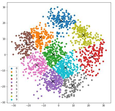
Visualizing the K-means clustering for handwritten data
- Plotting the k-means cluster using the scatter function provided by the matplotlib module.
- Reducing the large dataset by using Principal Component Analysis (PCA) and fitting it to the previously defined k-means++ model.
- Plotting the clusters with different colors, a centroid was marked for each cluster.
from sklearn.decomposition import PCA
import numpy as np

# Reducing the dataset
pca = PCA(2)
reduced_data = pca.fit_transform(digits_data)
kmeans_cluster.fit(reduced_data)

# Calculating the centroids
centroids = kmeans_cluster.cluster_centers_
label = kmeans_cluster.fit_predict(reduced_data)
unique_labels = np.unique(label)

# plotting the clusters:
plt.figure(figsize=(8, 8))
for i in unique_labels:
    plt.scatter(reduced_data[label == i, 0],
                reduced_data[label == i, 1],
                label=i)
plt.scatter(centroids[:, 0], centroids[:, 1],
            marker='x', s=169, linewidths=3,
            color='k', zorder=10)
plt.legend()
plt.show()
Output:
You can download the source code from here.