

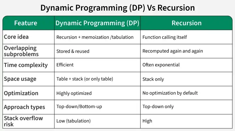
Dynamic Programming (DP) is an algorithmic technique used to solve complex problems by breaking them down into simpler overlapping subproblems. It is an optimization over plain recursion where we store the results of subproblems so that we do not have to re-compute them when needed later.
Recursion vs Dynamic Programming (DP)
How DP Works?
You should consider DP if a problem requires finding the maximum, minimum, or total number of ways, and you notice that you are repeating the same calculations over and over.
The Two Main Approaches:
- Top-Down (Memoization): This is the recursive approach. We start from the main problem and break it down. We use a table (usually an array or hash map) to store results. Before solving a subproblem, we check if it's already in our table.
- Bottom-Up (Tabulation): This is the iterative approach. We solve the smallest subproblems first and store their results in a table (usually a 1D or 2D array). We then use these results to solve larger and larger subproblems until we reach the final goal.
States and Transitions :
State :
A State is a set of variables that uniquely describe a subproblem like "snapshot". It must contain enough information to make future decisions without needing to know "how" you reached that state.
Example (0/1 Knapsack): The state is dp[i][w], where i is the number of items considered and w is the remaining capacity.
Transition:
A Transition is the logical rule or formula that connects one state to another. It defines how you move from subproblems to the main problem.
Example (0/1 Knapsack): To find dp[i][w], you decide: "Do I take item i or not?" : dp[i][w] = max(dp[i-1][w], val[i] + dp[i-1][w - wt[i]]).
Optimization Priority: Transitions vs. Space
Step 1: Transition Optimization (The Priority)
Always optimize the transition first. Reducing the complexity of how you compute a state often yields a better Time Complexity (e.g., from O(N^3) to O(N^2)).
- How? Using techniques like Sliding Window, Prefix Sums, or Segment Trees within your DP loops.
- Why? A faster program is usually more critical than a program that uses slightly less RAM.
Step 2: Space Optimization
Once your time complexity is optimal, look at the Space.
- How? If
dp[i]only depends ondp[i-1], you can replace a 2D array with two 1D rows (or even a single row updated in-place). - Why? This reduces space from O(N*W) to O(W).
Rule of Thumb: Focus on Transitions to pass the "Time Limit Exceeded" (TLE) error, and focus on Space to pass the "Memory Limit Exceeded" (MLE) error.
Classical Examples:
Nth Fibonacci Number
The Fibonacci series is a sequence where a term is the sum of previous two terms. The first two terms of the Fibonacci sequence are 0 followed by 1. The Fibonacci sequence: 0, 1, 1, 2, 3, 5, 8, 13, 21.
Instead of recalculating F(n) repeatedly, DP memoizes results in a table. The algorithm checks the table first: if a value exists, it retrieves it instantly; otherwise, it computes, stores, and returns it, reducing complexity from O(2^n) to O(n).
#include <iostream>
#include <vector>
using namespace std;

int nthFibonacci(int n){

    // base cases
    if (n <= 1)
        return n;

    vector<int> dp(n + 1);
    dp[0] = 0; dp[1] = 1;

    // solving the smaller problems first
    // and finally solving the complete problem
    for (int i = 2; i <= n; i++) {
        dp[i] = dp[i - 1] + dp[i - 2];
    }
    return dp[n];
}

int main(){
    int n = 5;
    int result = nthFibonacci(n);

    cout << result << endl;

    return 0;
}
class GFG {
    static int nthFibonacci(int n) {
        // base cases
        if (n <= 1) return n;

        int[] dp = new int[n + 1];

        dp[0] = 0;
        dp[1] = 1;

        // solving the smaller problems first
        // and finally solving the complete problem
        for (int i = 2; i <= n; ++i) {
            dp[i] = dp[i - 1] + dp[i - 2];
        }

        return dp[n];
    }

    public static void main(String[] args) {
        int n = 5;
        int result = nthFibonacci(n);
        System.out.println(result);
    }
}
# code
print("GFG")
def nthFibonacci(n):

    if n <= 1:
        return n

    dp = [0] * (n + 1)

    dp[0], dp[1] = 0, 1

    # solving the smaller problems first
    # and finally solving the complete problem
    for i in range(2, n + 1):
        dp[i] = dp[i - 1] + dp[i - 2]

    return dp[n]

if __name__ == "__main__":
    n = 5
    result = nthFibonacci(n)
    print(result)
using System;

class GFG {
    public static int nthFibonacci(int n) {
        if (n <= 1) return n;

        int[] dp = new int[n + 1];

        dp[0] = 0;
        dp[1] = 1;

        // solving the smaller problems first
        // and finally solving the complete problem
        for (int i = 2; i <= n; ++i) {
            dp[i] = dp[i - 1] + dp[i - 2];
        }

        return dp[n];
    }

    static void Main() {
        int n = 5;
        int result = nthFibonacci(n);
        Console.WriteLine(result);
    }
}
function nthFibonacci(n) {

    // base cases
    if (n <= 1) return n;

    let dp = new Array(n + 1);
    dp[0] = 0;
    dp[1] = 1;

    // solving the smaller problems first
    // and finally solving the complete problem
    for (let i = 2; i <= n; i++) {
        dp[i] = dp[i - 1] + dp[i - 2];
    }
    return dp[n];
}

// Driver code
let n = 5;
let result = nthFibonacci(n);
console.log(result);
Output
5
Time Complexity: O(n), each fibonacci number is calculated only one time,
Auxiliary Space: O(n), for dp table.
Given two arrays, profit[] and weight[], where each element represents the profit and weight of an item respectively, also given an integer W representing the maximum capacity of the knapsack (the total weight it can hold).
Put the items into the knapsack such that the sum of profits associated with them is the maximum possible, without exceeding the capacity W.
Note: We can either include an item completely or exclude it entirely - we cannot include a fraction of an item.
To compute the current row of the dp[] array, we only need values from the previous row. Therefore, instead of maintaining the entire 2D dp table, we can optimize space by using just a single 1D array. By traversing the array from right to left, we ensure that previously computed values are not overwritten before they are used.
#include <iostream>
#include<vector>
using namespace std;
//Driver Code Ends

int knapsack(int W, vector<int> &val, vector<int> &wt) {
    int n = wt.size();
    vector<vector<int>> dp(n + 1, vector<int>(W + 1));

    // Build table dp[][] in bottom-up manner
    for (int i = 0; i <= n; i++) {
        for (int j = 0; j <= W; j++) {

            // If there is no item or the knapsack's capacity is 0
            if (i == 0 || j == 0)
                dp[i][j] = 0;
            else {
                int pick = 0;

                // Pick ith item if it does not exceed the capacity of knapsack
                if(wt[i - 1] <= j)
                    pick = val[i - 1] + dp[i - 1][j - wt[i - 1]];

                // Don't pick the ith item
                int notPick = dp[i - 1][j];

                dp[i][j] = max(pick, notPick);
            }
        }
    }
    return dp[n][W];
}

//Driver Code Starts
int main() {
    vector<int> val = {1, 2, 3};
    vector<int> wt = {4, 5, 1};
    int W = 4;

    cout << knapsack(W, val, wt) << endl;
    return 0;
}
//Driver Code Ends
class GfG {
//Driver Code Ends

    static int knapsack(int W, int[] val, int[] wt) {
        int n = wt.length;
        int[][] dp = new int[n + 1][W + 1];

        // Build table dp[][] in bottom-up manner
        for (int i = 0; i <= n; i++) {
            for (int j = 0; j <= W; j++) {

                // If there is no item or the knapsack's capacity is 0
                if (i == 0 || j == 0)
                    dp[i][j] = 0;
                else {
                    int pick = 0;

                    // Pick ith item if it does not exceed the capacity of knapsack
                    if (wt[i - 1] <= j)
                        pick = val[i - 1] + dp[i - 1][j - wt[i - 1]];

                    // Don't pick the ith item
                    int notPick = dp[i - 1][j];

                    dp[i][j] = Math.max(pick, notPick);
                }
            }
        }
        return dp[n][W];
    }

//Driver Code Starts
    public static void main(String[] args) {
        int[] val = {1, 2, 3};
        int[] wt = {4, 5, 1};
        int W = 4;

        System.out.println(knapsack(W, val, wt));
    }
}
def knapsack(W, val, wt):
    n = len(wt)
    dp = [[0 for _ in range(W + 1)] for _ in range(n + 1)]

    # Build table dp[][] in bottom-up manner
    for i in range(n + 1):
        for j in range(W + 1):

            # If there is no item or the knapsack's capacity is 0
            if i == 0 or j == 0:
                dp[i][j] = 0
            else:
                pick = 0

                # Pick ith item if it does not exceed the capacity of knapsack
                if wt[i - 1] <= j:
                    pick = val[i - 1] + dp[i - 1][j - wt[i - 1]]

                # Don't pick the ith item
                notPick = dp[i - 1][j]

                dp[i][j] = max(pick, notPick)

    return dp[n][W]

if __name__ == "__main__":
#Driver Code Starts
    val = [1, 2, 3]
    wt = [4, 5, 1]
    W = 4

    print(knapsack(W, val, wt))
using System;
using System.Linq;

class GfG {
//Driver Code Ends

    static int knapsack(int W, int[] val, int[] wt) {
        int n = wt.Length;
        int[,] dp = new int[n + 1, W + 1];

        // Build table dp[][] in bottom-up manner
        for (int i = 0; i <= n; i++) {
            for (int j = 0; j <= W; j++) {

                // If there is no item or the knapsack's capacity is 0
                if (i == 0 || j == 0)
                    dp[i, j] = 0;
                else {
                    int pick = 0;

                    // Pick ith item if it does not exceed the capacity of knapsack
                    if (wt[i - 1] <= j)
                        pick = val[i - 1] + dp[i - 1, j - wt[i - 1]];

                    // Don't pick the ith item
                    int notPick = dp[i - 1, j];

                    dp[i, j] = Math.Max(pick, notPick);
                }
            }
        }
        return dp[n, W];
    }

//Driver Code Starts
    static void Main() {
        int[] val = { 1, 2, 3 };
        int[] wt = { 4, 5, 1 };
        int W = 4;

        Console.WriteLine(knapsack(W, val, wt));
    }
}
function knapsack(W, val, wt) {
    let n = wt.length;
    let dp = Array.from({ length: n + 1 }, () => Array(W + 1).fill(0));

    // Build table dp[][] in bottom-up manner
    for (let i = 0; i <= n; i++) {
        for (let j = 0; j <= W; j++) {

            // If there is no item or the knapsack's capacity is 0
            if (i === 0 || j === 0)
                dp[i][j] = 0;
            else {
                let pick = 0;

                // Pick ith item if it does not exceed the capacity of knapsack
                if (wt[i - 1] <= j)
                    pick = val[i - 1] + dp[i - 1][j - wt[i - 1]];

                // Don't pick the ith item
                let notPick = dp[i - 1][j];

                dp[i][j] = Math.max(pick, notPick);
            }
        }
    }
    return dp[n][W];
}

// Driver code
//Driver Code Starts
let val = [1, 2, 3];
let wt = [4, 5, 1];
let W = 4;

console.log(knapsack(W, val, wt));
Output
3
Time Complexity: O(n*W), as we fill a table of size (n+1)*(W+1).
Auxiliary Space: O(n*W), to store the 2D dp table.
Why Greedy Fails here ?
In the 0/1 Knapsack problem, the Greedy approach fails because it makes decisions based on immediate local gains (like the highest profit or the best profit-to-weight ratio) without considering how that choice limits future possibilities.
Unlike the Fractional Knapsack where you can "fill the gaps" with pieces of items, the 0/1 constraint means a single greedy choice can waste capacity that could have been used more efficiently by a combination of other items.
Common Algorithms that Use DP:
- Longest Common Subsequence (LCS): This is used in day to day life to find difference between two files (diff utility)
- Edit Distance : Checks how close to strings are. Can we be useful in implementing Google's did you mean type feature.
- Longest Increasing Subsequence : There are plenty of variations of this problem that arise in real world.
- Bellman–Ford Shortest Path: Finds the shortest path from a given source to all other vertices.
- Floyd Warshall : Finds shortest path from every pair of vertices.
- Knapsack Problem: Determines the maximum value of items that can be placed in a knapsack with a given capacity.
- Matrix Chain Multiplication: Optimizes the order of matrix multiplication to minimize the number of operations.
- Fibonacci Sequence: Calculates the nth Fibonacci number.
Advantages of Dynamic Programming (DP)
Dynamic programming has a wide range of advantages, including:
- Avoids recomputing the same subproblems multiple times, leading to significant time savings.
- Ensures that the optimal solution is found by considering all possible combinations.
Applications of DP
DP is used in various fields where optimization is key:
- Strings: Longest Common Subsequence, Edit Distance, Palindrome Partitioning.
- Knapsack Problems: 0/1 Knapsack, Partition equal subset sum.
- Graphs: Bellman-Ford algorithm (Shortest path), Floyd-Warshall (All-pairs shortest path).
- Mathematics: Fibonacci numbers, Pascal’s Triangle, Counting ways to reach a target.
Greedy vs Dynamic Programming (DP)
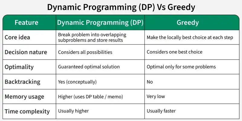
Greedy is faster but limited, DP is slower but always correct (for problems with overlapping subproblems).