

Color correction is an image processing technique used to correct color imbalances and improve the overall appearance of an image. It helps produce more natural and visually accurate colors. Common Color Correction Techniques include:
1. Histogram Equalization
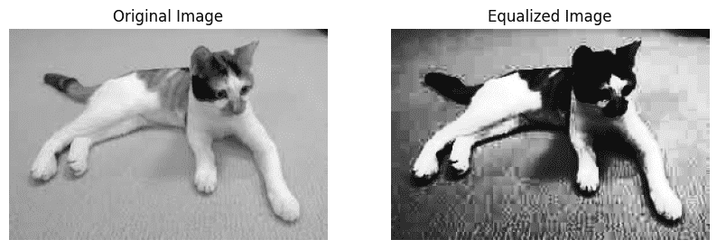
Histogram Equalization enhances image contrast by redistributing pixel intensity values, making details more visible in low-contrast regions.
- Load the image using cv2.imread().
- Convert the image to grayscale using cv2.cvtColor().
- Apply histogram equalization using cv2.equalizeHist().
- Display the enhanced image.
- Wait for a keyboard event before closing the window.
import cv2
import matplotlib.pyplot as plt

img = cv2.imread('/content/cat img.jpeg')

gray = cv2.cvtColor(img, cv2.COLOR_BGR2GRAY)

equalized = cv2.equalizeHist(gray)

plt.figure(figsize=(10, 5))

plt.subplot(1, 2, 1)
plt.imshow(gray, cmap='gray')
plt.title("Original Image")
plt.axis('off')

plt.subplot(1, 2, 2)
plt.imshow(equalized, cmap='gray')
plt.title("Equalized Image")
plt.axis('off')

plt.show()
Output:
2. Colour Space Conversion
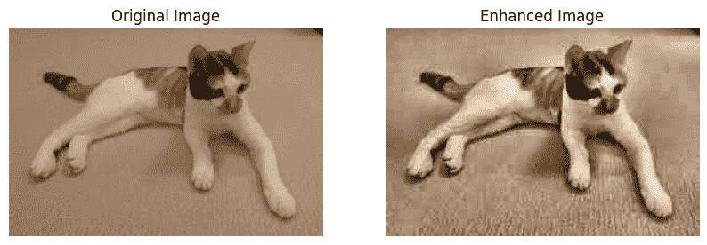
Color Space Conversion changes an image from one color space to another to improve color quality and contrast. In this technique, the image is converted from BGR to LAB color space, enhanced using CLAHE and then converted back to BGR.
- Load the input image.
- Convert the image from BGR to LAB color space.
- Apply CLAHE to the L channel.
- Merge the channels and convert the image back to BGR.
- Display the enhanced image.
import cv2
import matplotlib.pyplot as plt

img = cv2.imread('image path')

lab = cv2.cvtColor(img, cv2.COLOR_BGR2LAB)

l, a, b = cv2.split(lab)

clahe = cv2.createCLAHE(clipLimit=3.0, tileGridSize=(8, 8))
l = clahe.apply(l)

lab = cv2.merge((l, a, b))
output = cv2.cvtColor(lab, cv2.COLOR_LAB2BGR)

img_rgb = cv2.cvtColor(img, cv2.COLOR_BGR2RGB)
output_rgb = cv2.cvtColor(output, cv2.COLOR_BGR2RGB)

plt.figure(figsize=(10, 5))

plt.subplot(1, 2, 1)
plt.imshow(img_rgb)
plt.title("Original Image")
plt.axis('off')

plt.subplot(1, 2, 2)
plt.imshow(output_rgb)
plt.title("Enhanced Image")
plt.axis('off')

plt.show()
Output:
3. Image Filtering
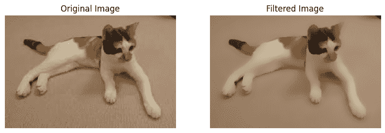
Image Filtering is used to reduce noise and improve image quality while preserving important details. In this example, a bilateral filter is applied to smooth the image while maintaining edge information.
- Load the input image using cv2.imread().
- Apply a bilateral filter using cv2.bilateralFilter().
- Display the filtered image and compare it with the original image.
import cv2
import matplotlib.pyplot as plt

img = cv2.imread('image.jpg')

filtered = cv2.bilateralFilter(img, 15, 75, 75)

img_rgb = cv2.cvtColor(img, cv2.COLOR_BGR2RGB)
filtered_rgb = cv2.cvtColor(filtered, cv2.COLOR_BGR2RGB)

plt.figure(figsize=(10, 5))

plt.subplot(1, 2, 1)
plt.imshow(img_rgb)
plt.title("Original Image")
plt.axis('off')

plt.subplot(1, 2, 2)
plt.imshow(filtered_rgb)
plt.title("Filtered Image")
plt.axis('off')

plt.show()
Output:
Download full code from here
Applications
- Improves the visual quality of photographs and digital images.
- Enhances medical and satellite images for better analysis.
- Used in image editing, photography and graphic design.
- Helps improve image quality in computer vision and machine learning applications.
- Corrects color imbalances caused by lighting or camera settings.
Advantages
- Improves image contrast and color balance automatically.
- Enhances the visibility of image details.
- Reduces the need for manual image adjustments.
- Produces more natural and visually appealing images.
- Can be efficiently implemented using OpenCV and Python.
Limitations
- Results may vary depending on image quality and lighting conditions.
- Excessive correction can produce unnatural colors.
- Some techniques may increase image noise or artifacts.
- Different images may require different correction parameters.
- Automatic methods may not always achieve the desired visual appearance.